
Explanations and implied causal mechanisms for digital media use often operate at the individual level. For example, the hypothesis photo sharing with friends increases social connectedness implies that when people share more photos they will feel more connected. A typical test of such a hypothesis might rely on a linear regression with a count measure for average number of photos shared with friends on a typical day as the independent variable, and an ordinal 7-point self-report scale for perceived social connectedness. If the resulting beta is positive and significant, let’s say 0.2, this would indicate that on average, an increase of one photo shared is associated with a 0.2 increase in connectedness, lending support for the hypothesis.

The problem: the hypothesis is not specific enough and all the data can show is that photo sharing and connectedness are positively associated at the between-person level. I recently asked students to think about the relationship between typing speed and error rate on a computer keyboard (see slide from the course below; the example is originally from Loes Keijsers). Thankfully, the exercise worked perfectly: the first student said she would expect there to be a positive relationship, since when you start typing faster, you’re probably going to make more mistakes; the second student then mentioned she would expect the opposite, since she types much faster than her grandma but still makes fewer mistakes. Thus, there are two very plausible explanations, yet they imply exactly the opposite relationship.
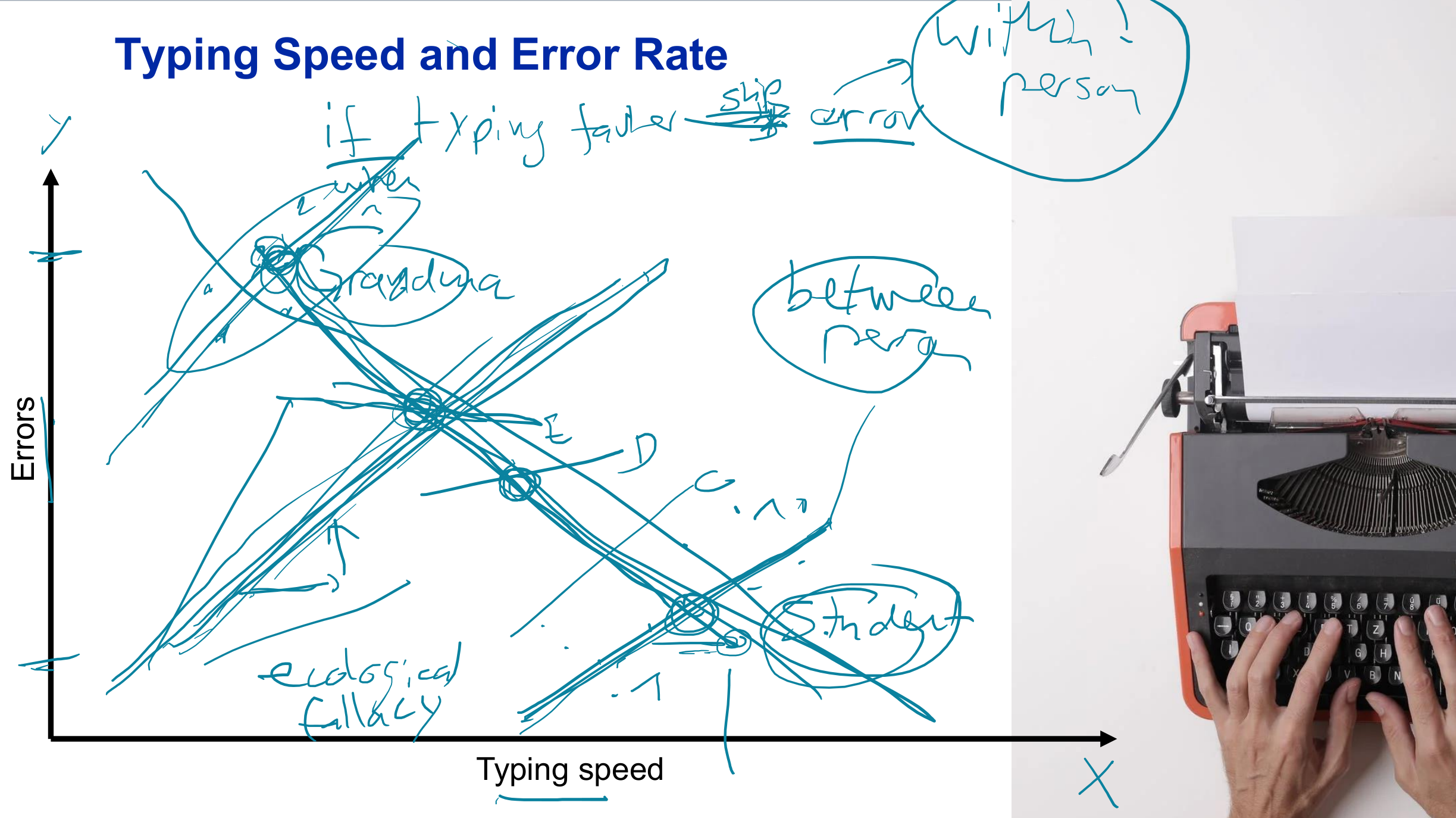
- At the between-person level, the association is expected to be negative: faster typists tend to make fewer mistakes than slow typists (because of their typing proficiency). The question is, who makes more errors? (Answer: on average, those who type slow).
- At the within-person level, the association is expected to be positive: when a typist increases their speed, they will make more errors (than usual). The question is, when do people make more errors? (Answer: on average, when they type fast).
Accordingly, it would be incorrect to conclude from cross-sectional data and a between-person analysis that typing speed decreases errors (and that people should thus just speed up if they want to make fewer errors).
Going back to the example of photo sharing, the explanations may be less clear but the same issue arises. Intuitively, we would probably expect the two to be positively associated, since when you share more photos with friends, you then feel more connected. But maybe individuals at moments in their life when they feel particularly disconnected from others then increase their photo sharing (which switches the cause and effect, and with it, the expected association). Though not sufficient, an empirical test of a causal mechanism at the individual level requires multiple measurements for each person.
Simulation in R
To visualize how aggregate-level bivariate associations may mask associations nested within individuals, we can simulate data in R. The setup specifies the number of individuals (here n=3) and the number of repeated measures (let’s set rm=100; so imagine e.g., participants get asked twice a day for 50 days how many photos they shared and how connected they feel). Then, each person’s overall mean needs to be set on both variables (x1 and x2), in this example in such a way that they are somewhat positively correlated. For simplicity, let’s also assume both variables are measured on a 1 to 10 scale.
n <- 3 # number of individuals
rm <- 100 # number of repeated measures
ni <- n * rm # number of data points

set.seed(42) # use only if you want the results to be reproducible

library(truncnorm) # modified version of rnorm() to allow min and max specification

# set means
imeansx1 <- c(2.9, 5.8, 7.7)
imeansx2 <- c(2.5, 4.1, 5.6)

# set std deviations
isdsx1 <- c(1.9, 2.3, 1.2)
isdsx2 <- c(2.1, 2.0, 1.9)

# set range of the variables
scalemin <- 1
scalemax <- 10

#
Now the actual values (300 in total) can be randomly drawn from a truncated (to avoid values outside the possible range) normal distribution. Then we can have a look at the distributions of each variable as well as their relationship.
x1 <- rtruncnorm(ni, mean = imeansx1, sd = isdsx1,
                 a = scalemin, b = scalemax)
x2 <- rtruncnorm(ni, mean = imeansx2, sd = isdsx2,
                 a = scalemin, b = scalemax)
hist(x1)
hist(x2)
plot(x1,x2)
cor(x1,x2)

Both variables are at least somewhat normally distributed around the specified means, and because of the set up, we can observe the positive association between x1 and x2 (here, the correlations coefficient was 0.44, which would be identical to beta in a linear regression for this bivariate case). However, this scatterplot disregards the nested structure of the data; there are 300 dots in the plot, but these need to be disaggregated by the three individuals.
After some data prep and ggplot2 code, we can look at the data in this way. The gray dashed line indicates the global fit. Each person now is assigned a color and a shape, and gets their own fit line. The whole simulation can be run many times, and sometimes all three colored lines will be positive, or all of them negative, or a mixture.
# create variable to identify individuals A, B, C
Person <- rep(LETTERS[1:n], rm)

df <- as.data.frame(cbind(Person,x1,x2))
df$Person <- as.factor(df$Person)
df$x1 <- as.numeric(df$x1)
df$x2 <- as.numeric(df$x2)

# i means sampled (vs. specfified distribution means)
aggregate(x = df$x1, by = list(df$Person), FUN = mean); imeansx1
aggregate(x = df$x2, by = list(df$Person), FUN = mean); imeansx2


# compare individual fit lines with global fit lines
library(ggplot2)

## x2 ~ x1
ggplot(df, aes(x = x1, y = x2)) +
  geom_point(aes(shape = Person, color = Person)) +
  geom_smooth(method = "lm", formula = y ~ x, se = F,
              color = "#bfbfbf", linetype = "longdash") + # global fit
  geom_smooth(aes(color = Person), method = "lm", formula = y ~ x, se = F) + # individual fit
  scale_color_manual(values=c('#75d9d4','#d264e3', '#e3bf64')) +
  theme(legend.position="top") +
  guides(color = guide_legend(override.aes = list(size = 0.5))) +
  theme(panel.grid.major = element_blank(), panel.grid.minor = element_blank(),
        panel.background = element_blank(), axis.line = element_line(colour = "black")) +
  theme(legend.position = "none")

#

One thought on “Analyzing Between-Person and Within-Person Associations”